Mario Coiro

In my short research career I have become more and more intersted in how to appropriately represent uncertainty in phylogenetic analyses.

Phylogenetic trees based on morphology are often represented as a single (strict or majority) consensus tree, sometimes with branches labelled with branch support (bootstrap/jackknife percentages or ‘Decay index’). However, in many cases this form of representation does not appropriately illustrate the structure of the underlying phylogenetic signal.

For example, low bootstrap support for a clade (or low posterior probability) can indicate either the absence of singal supporting that particular grouping or the presence of a strong conflicting signal. In both these cases, the consensus tree can be identical, but the implications of the data for further investigations is rather different.

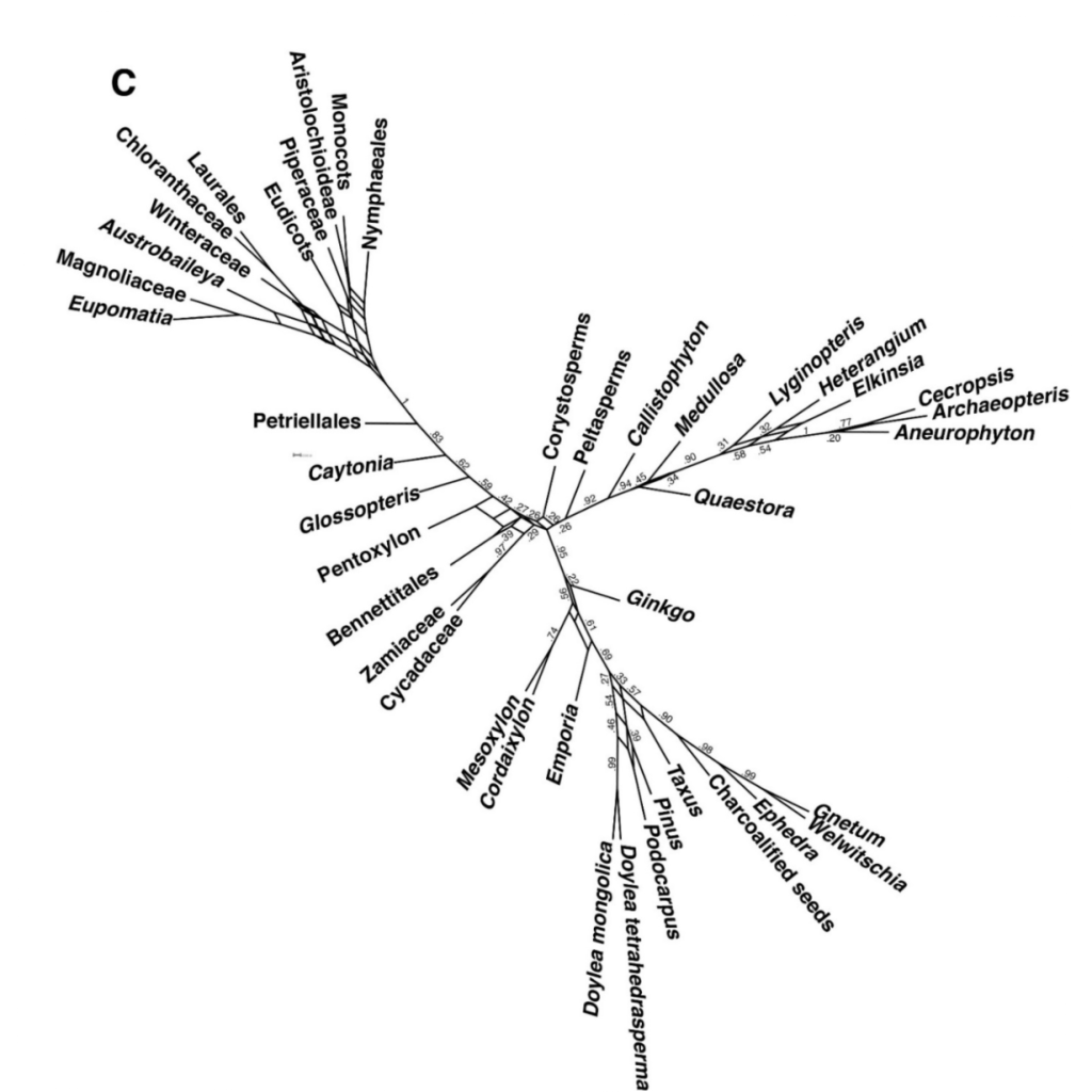
One way of better representing the information in a bootstrap replicate or a posterior sample from a Bayesian analysis is to use consensus networks. These graphs are incredibly easy to obtain (using the software SplitsTree), and they are extremely informative. Moreover, Guido Grimm, the person that inspired me to use this tool in the first place, and has fought for a long time for better practices in analysing and representing phylogenetic signal, has extensively treated why these graphs are often better than consensus trees and how to build them (here, here, and here for example).

We have used them to great results in our analyses on the signal of morphology in the phylogeny of seed plants (you can find it here). However, these graphs are often not that easy to read for people who are not used to them.

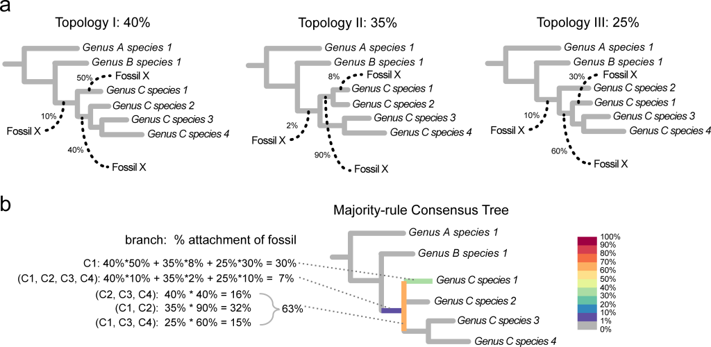
An alternative to consensus networks is the use of RoguePlots, a method elaborated by Seraina Klopfstein and Tamara Spasojevic and implemented as a library in R.  These graphs are particuarly advantageous for situations where one of few fossil taxa are placed on a ‘backbone’ topology derived from molecular or other analyses, a practice which is quite common for fragmentary plant fossils. However, they work well for any kind of analysis.

RoguePlots represent the uncertainty of the placement of one taxon at the time (the rogue) on a partially resolved tree (usually a consensus tree, or a backbone tree). This is done by color-coding the differet branches on a consensus or backbone tree by the percentage of the trees in a sample (bootstrap or posterior, depending on the anlayses) that present the rogue taxon in that particular position, while placements in clades that are not present in the consensus are indicated by coloring the vertical bars of the tree. This is visually pretty similar (though not entirely equivalent) to the common usage of color-coded branches to indicate the number of parsimony steps different from the most-parsimonious position used in many paleobotanical papers (and brilliantly applied to flowers on a massive angiosperm phylogeny and automated by Schönenberger et al. 2020).

So, how does one build a RoguePlot?

Fortunately, it is extremely easy. You are going to need R, a consensus or backbone tree in either newick or nexus format and the posterior sample of the trees from your Bayesian analysis or bootstrap replicates from Parsimony or Maximum Likelihood analysis.

We will use our analyses from our recent paper on Mesodescolea as an example here. You are going to need the files here to run this code.

You first need to install the RoguePlots library and load it. This can be done by downloading the windows complied version from GitHub or using the install_github function from the package devtools.

if(!require(devtools)){install.packages("devtools")}; library(devtools)
install_github('seraklop/RoguePlots/rogue.plot'); library(rogue.plot)

You then need to load the consensus tree (or the backbone tree). In our case, it’s the backbone tree with the topology from the Li et al. (2019) analysis (‘Lietal.nex’). You also need to load the bootstrap or posterior trees. In our case, the posterior trees from our bayesian analyses have been combined in a single file (‘Li_et_al_BIposterior.t’) after removing the first 25% (the burn-in fraction).

#Read the consensus tree
tree = read.nexus('Lietal.nex') #tree in nexus format
#tree = read.tree('tree') #tree in pyhlip format

#Read the posterior trees or the bootstrap trees 
reftrees = read.nexus('Li_et_al_BIposterior.t')#tree in nexus format

You then need to specify the name of the rogue or rogues. In our case, since the backbone tree does not contain our rogue, the analysis would work even without specifying the rogue.

rogues = 'Mesodescolea' #name of the rogue

You then use the function create.rogue.plot, adding the backbone/consensus tree, the bootstrap/posterior trees, the names of your rogue (you can omit this if the rogues are not in your backbone tree), as well as the name of the outgroup (Amborella in our case), plus a few graphical options and the names for the two files this function will produce: a table including the name of the rogue, the different placement of your rogue (indicated as lists of taxa that you rogue is ‘sister’ to), the frequency, and whether these groups are present in the consensus/backbone tree; and a pdf graph with the placements of you rogue indicated on the consensus or backbone tree with different degrees of gray (or the color scale of your choice).

create.rogue.plot(tree, reftrees,rogues,  outgroup = 'Amborella', type = 'greyscale', col = NULL,
outfile.table = 'table.txt', outfile.plot = 'graph.pdf', min.prob = 0.01, cex.tips = par('cex'), tip.color = 'black')

And here is the resulting graph for our example:

This shows that Mesodescolea is placed mostly somewhere in Austrobaileyales by Bayesian analyses, with some trees in the sample indicating a placement in Chloranthaceae. With a bit of polishing using a vectorial editing software, we got to the figures used in our manuscript.

I am really grateful to Seraina Klopfstein for introducing me to RoguePlots, and I plan to appy them quite widely in the future. I hope this tutorial and explanation will push more people (especially paleobotanists) to adopt these methods more widely!

References:

Coiro, M., Chomicki, G. and Doyle, J.A., 2018. Experimental signal dissection and method sensitivity analyses reaffirm the potential of fossils and morphology in the resolution of the relationship of angiosperms and Gnetales. Paleobiology, 44(3), pp.490-510.

Klopfstein, S. and Spasojevic, T., 2019. Illustrating phylogenetic placement of fossils using RoguePlots: An example from ichneumonid parasitoid wasps (Hymenoptera, Ichneumonidae) and an extensive morphological matrix. PloS one, 14(4), p.e0212942.

Li, H.T., Yi, T.S., Gao, L.M., Ma, P.F., Zhang, T., Yang, J.B., Gitzendanner, M.A., Fritsch, P.W., Cai, J., Luo, Y. and Wang, H., 2019. Origin of angiosperms and the puzzle of the Jurassic gap. Nature Plants, 5(5), pp.461-470.

Rothwell, G.W. and Stockey, R.A., 2016. Phylogenetic diversification of Early Cretaceous seed plants: The compound seed cone of Doylea tetrahedrasperma. American Journal of Botany, 103(5), pp.923-937.

Schönenberger, J., von Balthazar, M., López Martínez, A., Albert, B., Prieu, C., Magallón, S. and Sauquet, H., 2020. Phylogenetic analysis of fossil flowers using an angiosperm‐wide data set: proof‐of‐concept and challenges ahead. American Journal of Botany, 107(10), pp.1433-1448.